Centering covariance matrices

Corson N. Areshenkoff

2024-10-01

My own neuroimaging work frequently uses covariance centering in order to isolate specific task changes in fMRI functional connectivity, or to filter out baseline subject differences. The mechanics underlying this centering are fairly complex, but spdm provide a convenient a flexible wrapper function for centering covariance matrix valued data using the spd.center() function.

Tutorial

spdm includes a sample neuroimaging dataset containing standardized BOLD timecourses from 5 subjects in each of 5 different conditions. This dataframe contains fields for Subject and Condition, as well as a Data field containing a list of matrices (n_timepoints x n_regions).

In a simple workflow, we might begin by computing the covariance between each of these timecourses:

data(bold)
names(bold)
#> [1] "Subject"   "Condition" "Data"

# Note that it is almost always better to use some kind of regularized
# covariance estimate, but we will use the sample covariance here for 
# illustration. For higher dimensional problems, it is likely that the 
# sample covariance will not be positive definite.
covmats <- lapply(bold$Data, spd.estimate, method = "sample")

As a visualization aid, it is sometimes useful to create some kind of low-dimensional representation of the data. Multidimensional scaling will do in this case, and we’ll construct the distance matrix using the pairwise geodesic distances between covariance matrix. At the moment, spd.dist only computes distance between a single pair (i.e. not in bulk), and so we’ll borrow from the proxy packages in order to compute these efficiently:

D_uncentered <- proxy::dist(covmats, method = function(i,j) 
    spd.dist(i, j, method = "riemannian"))
mds_uncentered <- cmdscale(D_uncentered)

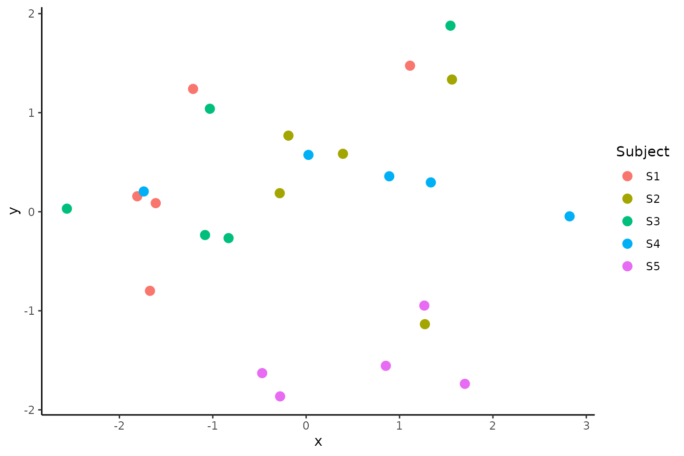
If we plot the embedded covariance matrices colored by subject we see a phenomenon which has been widely replicated in the neuroimaging literature: the clustering of covariance matrices within subjects:

plot_data <- data.frame(Subject = bold$Subject,
                        x = mds_uncentered[,1],
                        y = mds_uncentered[,2])
ggplot(plot_data, aes(x = x, y = y, color = Subject)) +
    geom_point(size = 3) + theme_classic()

That is, functional connectivity measured in the same subject under different task conditions is more similar than the same task condition measured in different subjects (see Gratton et al. 2018). In fact, this finding can be replicated under fairly extreme conditions; for example, in Areshenkoff et al.  (2021) we find similar clustering in Macaques under different doses of anesthesia. This is true even when comparing nearly awake scans to those in which the animal is totally sedated.

The actual cause of this clustering is debated, but there are likely two general reasons: 1) Functional connectivity is strongly constrained by structural connectivity, which is variable across subjects; and 2) Group average parcellations do not capture functional heterogeneity in the cortex, so (for very fine parcellations) the same parcel of cortex has slightly different functions across subjects.

Either way, the result is that actual task differences in functional connectivity are buried in much larger static inter-subject differences. A sensible strategy in this case would be to remove average subject differences by “translating” the covariance matrices so that all subject means align with a common reference point (generally, the grand mean). This is quite simple with the spd.center() function, which accepts a dataframe of observation information, a list of covariance matrices, and various constraints defining the centering.

covmats_centered <- spd.center(d = bold, covmats = covmats, group_by = "Subject")

In this case, we only need to align the subjects, and so specifying group_by = "Subject" is enough.

centered_data <- spd.center(d = bold, covmats = covmats, group_by = 'Subject')
covmats_centered <- centered_data$centered_covmats

D_centered <- proxy::dist(covmats_centered, method = function(i,j) 
    spd.dist(i, j, method = 'riemannian'))
mds_centered <- cmdscale(D_centered)

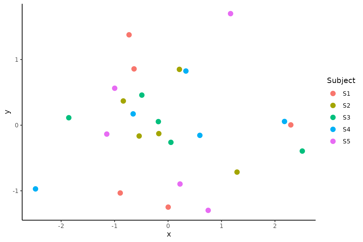
And now the subject clustering is abolished.

plot_data <- data.frame(Subject = bold$Subject,
                        x = mds_centered[,1],
                        y = mds_centered[,2])
ggplot(plot_data, aes(x = x, y = y, color = Subject)) +
    geom_point(size = 3) + theme_classic()

As a side note, many analyses are better conducted on the tangent vectors around the grand mean (that is, the centered covariance matrices projected onto the tangent space around the mean), and so spd.center() returns both the centered covariance matrices, and the target mean. The tangent vectors can then be easily computed by log-mapping the centered observations:

tanvecs <- lapply(centered_data$centered_covmats, spd.logmap, 
                  p = centered_data$target_covariance)

In some cases, the user is specifically interested in differences relative to some reference condition (e.g. a resting state scan), and so it may be preferable to center so that the reference scans for each subject are aligned to the
overall mean reference scan. For example, we might wish to align condition “A” in this dataset. In that case, constraints can be specified using the arguments from_constraints and to_constraints. In this case, we want to center to the mean of all observations in condition A, and so we set

from_constraints <- "Condition == 'A'"
to_constraints   <- "Condition == 'A'"

In the case of to_constraints, this condition is applied within subjects, so that we take only those observations in condition A when computing the subject means.

centered_data <- spd.center(d = bold, covmats = covmats, group_by = "Subject",
                            from_constraints = from_constraints,
                            to_constraints = to_constraints)
covmats_centered <- centered_data$centered_covmats

D_centered <- proxy::dist(covmats_centered, method = function(i,j) 
    spd.dist(i, j, method = 'riemannian'))
mds_centered <- cmdscale(D_centered)

plot_data <- data.frame(Subject = bold$Subject,
                        Condition = bold$Condition,
                        x = mds_centered[,1],
                        y = mds_centered[,2])
ggplot(plot_data, aes(x = x, y = y, color = Subject, shape = Condition)) +
    geom_point(size = 3, alpha = .5) + theme_classic()

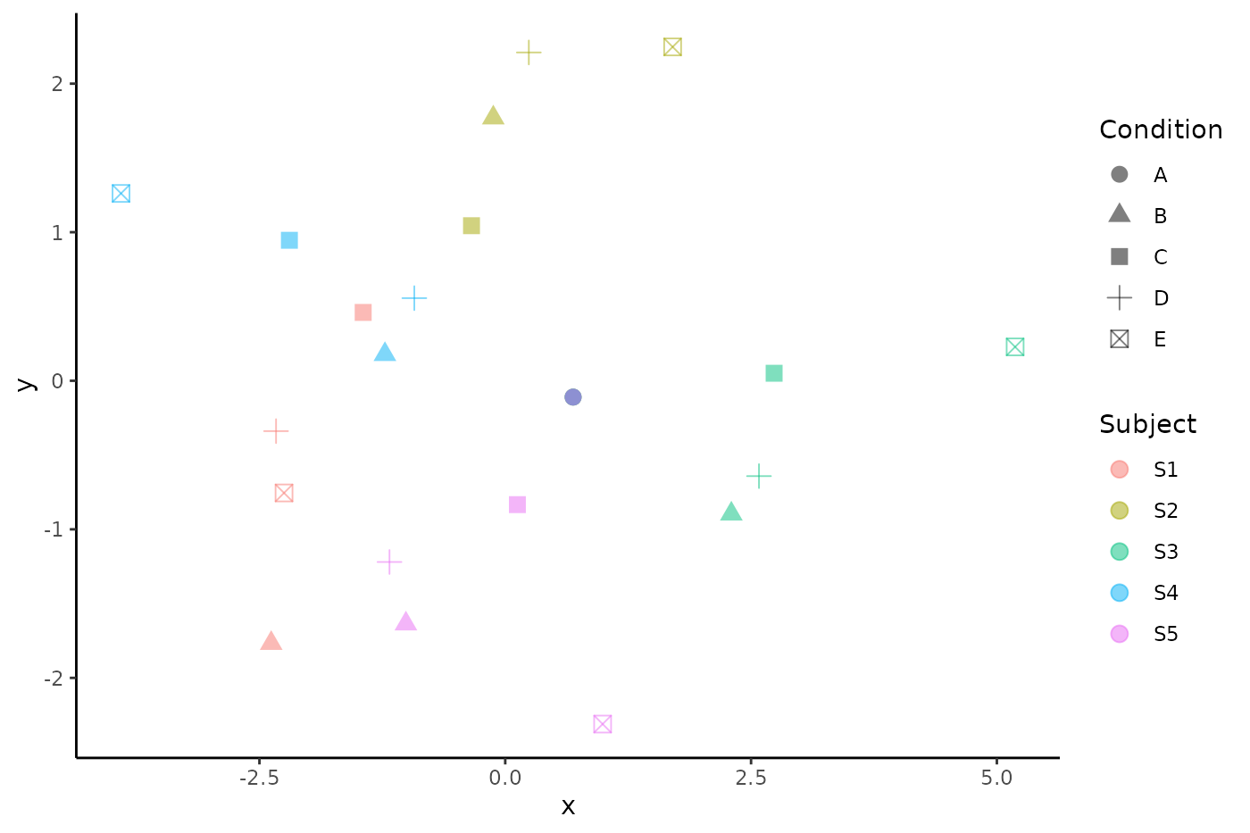
where we now have a cluster of identical observations at (0,0) for condition A, as these observations have been aligned across subjects. Note that this kind of centering has not succeeded in eliminating subject level clustering, since in addition to subject level differences, subject-by-task interactions also tend to be much larger than pure task effects.

Caveats

Although I intend to write a more formal description of this issue in the near future, covariance centering causes issues of interpretation that are worth discussing here at a high-level.

Given a covariance matrix \(\Sigma\), entry \((i,j)\) has an unambiguous interpretation as the covariance between variables \(i\) and \(i\). After centering by parallel transport – as in done by spd.center – the resulting entry \((i,j)\) in the centered matrix \(\bar{\Sigma}\) is actually a linear combination of the entries in \(\Sigma\), and so doesn’t necessary have an unambiguous interpretation in terms of the original variables. This problem is exacerbated when transporting over longer distances, which is the primary motivation for centering to the grand mean, since this value minimizes the average (squared) distance to the individual observations.

It is possible to explicitly quantify the contributions of each covariance to the value of the centered covariances; but there is no general, principled method of identifying how much overall distortion has occurred (although this is a major current interest of mine).

References

Areshenkoff, C. N., Nashed, J. Y., Hutchison, R. M., Hutchison, M., Levy, R., Cook, D. J., … & Gallivan, J. P. (2021). Muting, not fragmentation, of functional brain networks under general anesthesia. Neuroimage, 231, 117830.

Gratton, C., Laumann, T. O., Nielsen, A. N., Greene, D. J., Gordon, E. M., Gilmore, A. W., … & Petersen, S. E. (2018). Functional brain networks are dominated by stable group and individual factors, not cognitive or daily variation. Neuron, 98(2), 439-452.